A Appendix A: Development Plan

Algorithm incorporation
1. Joint pulses
  1. covariates
2. Population model
  1. covariates
Modularization/refactoring
Manual/webbook
Package features
1. Summary and diagnostic functions

A.1 Software map

Single subject
1. Single hormone
2. 2 hormones
- Options:
  - Orderstat vs Strauss
  - Changing baseline??
Population model
1. Single hormone
  - Single group (no covariates)
  - Covariates (> 1 group)
    - Choose which parameters to do as a regression (- categorical parameters; - continuous parameters), others under single group assumptions.
2. 2 hormones
  - Single group
    - non 1-to-1 (imperfect)
    - - 2 driver (method needed) (what does this mean?)
  - Covariates (> 1 group)
    - non 1-to-1, imperfect, ???pamm done (p), need v/nu?? (what does this mean?)
    - 2 driver (method needed) (what does this mean?)

A.2 Base code versions for github archiving

All variations

Major versions

Single-subject, single hormone
Single-subject, associational (2-hormone)
Population model, single hormone
Population model, covariates, single hormone
Population model, associational (2-hormone) hormone
Population model, covariates, associational (2-hormone) hormone

Minor versions

Fixed baseline vs. change-point baseline vs changing baseline (sinusoidal)
Orderstat vs. Strauss prior on pulse location
Log-normal vs. truncated t prior on mean mass/width
- Only truncated-t going forward
Inverse Wishart vs. half-Cauchy vs. Uniform prior on re_sd
- Only Uniform prior going forward

Questions

Terminology: driver/response OR trigger/response

Summary and diagnostic functions

mcmc_trace <- function() {}
mcmc_posteriors <- function() {}
mcmc_locations <- function() {}

STAN and other Bayesian R package functions to implement

Posterior predicted values/plot

rstanarm::posterior_predict()
rstanarm::ppc_dens_overlay()
rstanarm::ppc_intervals()

Posterior densities

rstanarm::mcmc_areas()

#--------------------------------------------
# STAN examples
#   Some examples http://mc-stan.org/bayesplot/
#--------------------------------------------
if (!require(bayesplot)) install.packages("bayesplot")

## Loading required package: bayesplot

## This is bayesplot version 1.4.0

## - Plotting theme set to bayesplot::theme_default()

## - Online documentation at mc-stan.org/bayesplot

if (!require(rstanarm)) install.packages("rstanarm")

## Loading required package: rstanarm

## Loading required package: Rcpp

## Loading required package: methods

## rstanarm (Version 2.17.3, packaged: 2018-02-17 05:11:16 UTC)

## - Do not expect the default priors to remain the same in future rstanarm versions.

## Thus, R scripts should specify priors explicitly, even if they are just the defaults.

## - For execution on a local, multicore CPU with excess RAM we recommend calling

## options(mc.cores = parallel::detectCores())

## - Plotting theme set to bayesplot::theme_default().

if (!require(ggplot2))  install.packages("ggplot2")

## Loading required package: ggplot2

library(bayesplot)
library(rstanarm)
library(ggplot2)

fit        <- stan_glm(mpg ~ ., data = mtcars)

## 
## SAMPLING FOR MODEL 'continuous' NOW (CHAIN 1).
## 
## Gradient evaluation took 5.4e-05 seconds
## 1000 transitions using 10 leapfrog steps per transition would take 0.54 seconds.
## Adjust your expectations accordingly!
## 
## 
## Iteration:    1 / 2000 [  0%]  (Warmup)
## Iteration:  200 / 2000 [ 10%]  (Warmup)
## Iteration:  400 / 2000 [ 20%]  (Warmup)
## Iteration:  600 / 2000 [ 30%]  (Warmup)
## Iteration:  800 / 2000 [ 40%]  (Warmup)
## Iteration: 1000 / 2000 [ 50%]  (Warmup)
## Iteration: 1001 / 2000 [ 50%]  (Sampling)
## Iteration: 1200 / 2000 [ 60%]  (Sampling)
## Iteration: 1400 / 2000 [ 70%]  (Sampling)
## Iteration: 1600 / 2000 [ 80%]  (Sampling)
## Iteration: 1800 / 2000 [ 90%]  (Sampling)
## Iteration: 2000 / 2000 [100%]  (Sampling)
## 
##  Elapsed Time: 0.475231 seconds (Warm-up)
##                0.391947 seconds (Sampling)
##                0.867178 seconds (Total)
## 
## 
## SAMPLING FOR MODEL 'continuous' NOW (CHAIN 2).
## 
## Gradient evaluation took 1.7e-05 seconds
## 1000 transitions using 10 leapfrog steps per transition would take 0.17 seconds.
## Adjust your expectations accordingly!
## 
## 
## Iteration:    1 / 2000 [  0%]  (Warmup)
## Iteration:  200 / 2000 [ 10%]  (Warmup)
## Iteration:  400 / 2000 [ 20%]  (Warmup)
## Iteration:  600 / 2000 [ 30%]  (Warmup)
## Iteration:  800 / 2000 [ 40%]  (Warmup)
## Iteration: 1000 / 2000 [ 50%]  (Warmup)
## Iteration: 1001 / 2000 [ 50%]  (Sampling)
## Iteration: 1200 / 2000 [ 60%]  (Sampling)
## Iteration: 1400 / 2000 [ 70%]  (Sampling)
## Iteration: 1600 / 2000 [ 80%]  (Sampling)
## Iteration: 1800 / 2000 [ 90%]  (Sampling)
## Iteration: 2000 / 2000 [100%]  (Sampling)
## 
##  Elapsed Time: 0.447735 seconds (Warm-up)
##                0.425246 seconds (Sampling)
##                0.872981 seconds (Total)
## 
## 
## SAMPLING FOR MODEL 'continuous' NOW (CHAIN 3).
## 
## Gradient evaluation took 1.7e-05 seconds
## 1000 transitions using 10 leapfrog steps per transition would take 0.17 seconds.
## Adjust your expectations accordingly!
## 
## 
## Iteration:    1 / 2000 [  0%]  (Warmup)
## Iteration:  200 / 2000 [ 10%]  (Warmup)
## Iteration:  400 / 2000 [ 20%]  (Warmup)
## Iteration:  600 / 2000 [ 30%]  (Warmup)
## Iteration:  800 / 2000 [ 40%]  (Warmup)
## Iteration: 1000 / 2000 [ 50%]  (Warmup)
## Iteration: 1001 / 2000 [ 50%]  (Sampling)
## Iteration: 1200 / 2000 [ 60%]  (Sampling)
## Iteration: 1400 / 2000 [ 70%]  (Sampling)
## Iteration: 1600 / 2000 [ 80%]  (Sampling)
## Iteration: 1800 / 2000 [ 90%]  (Sampling)
## Iteration: 2000 / 2000 [100%]  (Sampling)
## 
##  Elapsed Time: 0.435891 seconds (Warm-up)
##                0.419295 seconds (Sampling)
##                0.855186 seconds (Total)
## 
## 
## SAMPLING FOR MODEL 'continuous' NOW (CHAIN 4).
## 
## Gradient evaluation took 1.8e-05 seconds
## 1000 transitions using 10 leapfrog steps per transition would take 0.18 seconds.
## Adjust your expectations accordingly!
## 
## 
## Iteration:    1 / 2000 [  0%]  (Warmup)
## Iteration:  200 / 2000 [ 10%]  (Warmup)
## Iteration:  400 / 2000 [ 20%]  (Warmup)
## Iteration:  600 / 2000 [ 30%]  (Warmup)
## Iteration:  800 / 2000 [ 40%]  (Warmup)
## Iteration: 1000 / 2000 [ 50%]  (Warmup)
## Iteration: 1001 / 2000 [ 50%]  (Sampling)
## Iteration: 1200 / 2000 [ 60%]  (Sampling)
## Iteration: 1400 / 2000 [ 70%]  (Sampling)
## Iteration: 1600 / 2000 [ 80%]  (Sampling)
## Iteration: 1800 / 2000 [ 90%]  (Sampling)
## Iteration: 2000 / 2000 [100%]  (Sampling)
## 
##  Elapsed Time: 0.419634 seconds (Warm-up)
##                0.385577 seconds (Sampling)
##                0.805211 seconds (Total)

posterior  <- as.matrix(fit)

plot_title <- ggtitle("Posterior distributions with medians and 80% intervals")
mcmc_areas(posterior, pars = c("cyl", "drat", "am", "wt"), prob = 0.8) +
  plot_title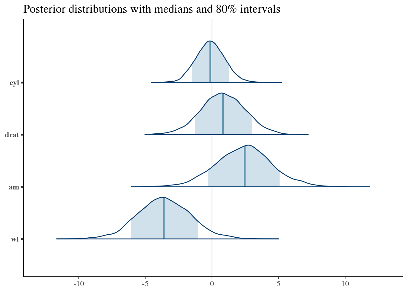

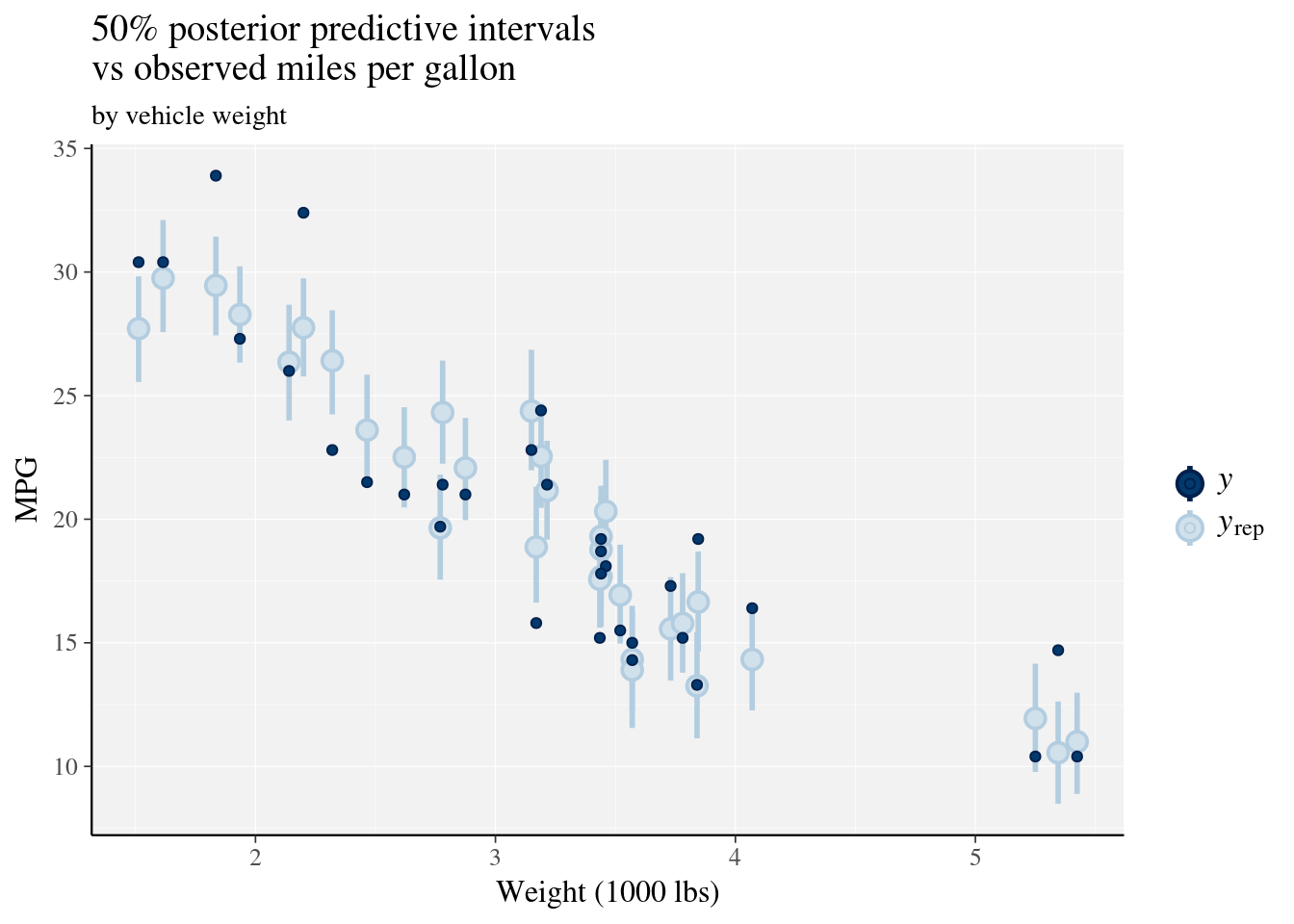
ppc_intervals(y = mtcars$mpg, yrep = posterior_predict(fit), x = mtcars$wt, prob = 0.5) +
  labs(x = "Weight (1000 lbs)",
       y = "MPG",
       title = "50% posterior predictive intervals \nvs observed miles per gallon",
       subtitle = "by vehicle weight") +
  panel_bg(fill = "gray95", color = NA) +
  grid_lines(color = "white")